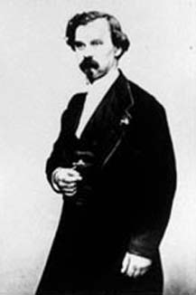
Jules
Antoine Lissajous (1822 - 1880)
Animation
The Maple command animate( ) provides us with new and exciting options. Imagine that F(x,t) is a function of x for each fixed value of t. Then
animate (F(x,t), x = c..d, t = e..f);
plots, for fixed t, the graph of F(x,t) on the interval c<x<d for a specified number of t-values evenly dispersed over the interval p<t<q. The default value for the number of t-values (each called a frame) is 16, but we can specify this number with the frames = n option. t is called the frame variable.
We will need the plots library to use animate. Consider the following example from our text.
> with(plots):
> animate(1/(1+x*t), x = 0..10, t = 0..1,
frames =10);
A plot of the constant function F(x,0) = 1 appears in the window (corresponding to the first t value of 0). Click on the plot. A new context bar appears containing a window for coordinates and nine new buttons. Try clicking each one to see its effect. These include:
Next, let us explore more examples.
> restart:
> with(plots):
> animate( m*x, x = -5..5, m = -40..40, frames
= 200, view = [-10..10,-100..100], color = GREEN, thickness=3);
In this example, we are graphing the straight line y
= mx for 200 different values of m, beginning at m = -40 and ending
at m = 40.
Note that the option view = [a..b, c..d]
produces a graph with a horizontal range a..b, and a vertical range of
c..d.
Next, consider an example involving a sine curve with changing frequency:
> animate(sin(x*t), x = 0..2*Pi, t = 1..9, frames = 50 , numpoints = 200);
Explain what is happening here. Does the amplitude of the sine
curve change as well?
Next consider:
> animate( sin(t)*sqrt(1-x^2), x = -1..1, t = 0..10*Pi, frames = 100, color = BLUE);
Note that y = sqrt(1-x2) is just a semi-circle of radius 1. What is the effect of the sin(t) coefficient?
For the next example, we will use polar coordinates. Note that another way to graph a curve in polar coordinates, r = r(theta), without using polarplot, is through the following command:
plot([r(theta), theta, theta = t0..t1], coords = polar);
For example:
> plot([5, theta, theta=0..10], coords = polar, filled = true);
graphs a circle of radius 5 centered at origin. Note that filled = true will color the circle.
> plot(sin(x), x = 0.. Pi, coords = polar);
graphs a circle of radius 1/2 centered at (0, 1/2).
To display an expanding circle, let the radius of a circle centered at the origin vary from 0 to 40. For example
> animate( [t, theta, theta = 0..2*Pi], t = 0..40, coords = polar );
(Unfortunately, the filled = true option seems not to be accepted by animate.)
The following is an animation of a multi-leaved rose (in polar coordinates):
> animate([sin(theta*t), theta, theta=-Pi..Pi], t=1..6, coords = polar, numpoints=200, frames=100, color=BLUE);
What happens if you change the range of values of the frame variable, t?
The following example of a Maple leaf is due to Professor G. Donald Allen, Department of Mathematics, Texas A&M University:
> s :=100/(100 + (theta - Pi/2)^8):
> r := s*(2 - sin(7*theta) - cos(30*theta)/2):
> animate([u*r/2, theta, theta = -Pi/2..3/2*Pi],
u = 1..2, numpoints=300, frames = 25, coords=polar, axes=none, color=GREEN
);
Next, let us consider the problem of the floating tangent line. That is, we wish to graph a function and its tangent line at x = t as t varies from t = a to t = b.
Let us begin with a particular function f(x) = sin x.
> graphSine := plot(sin(x), x = 0..2*Pi,-6.3..6.3, color=blue, thickness=2):
Using elementary calculus, the equation of the tangent line to f(x) at x = t is given by y = cos(t) (x-t) + sin(t). Hence:
> floatLine := animate(cos(t)*(x-t)+sin(t),
x = 0..2*Pi, t=0..2*Pi, frames=20, color=GREEN):
> display({floatLine, graphSine});
For homework, you will be asked to animate the floating tangent line for any differentiable function f(x).
Next, we will look at parametric curves and their animations.
For example, to graph a circle of radius 2 with center at (3, 5), we could
use parametric equations:
x = 3 + sin (theta) and y = 5 + cos (theta), letting theta vary from
0 to 2 Pi.
> plot ( [3 + sin(theta), 5 + cos(theta), theta = 0..2*Pi]);
The following animation displays a circle moving from left to right. What is the radius of the circle and what is the locus of its center?
animate([u+cos(theta), 1+sin(theta), theta=0..2*Pi], u=0..4*Pi, color=BLUE, view=[0..10, 0..10]);
Another way to animate an expanding circle would be to use parametric curves as follows:
> animate( [u*sin(t), u*cos(t), t = -Pi..Pi], u=1..8, view=[-8..8,-8..8]);
What happens if you change the range of u values?
Spirals can easily be described using polar coordinates: r = theta, for example.
> plot([theta, theta, theta=0..19], coords=polar);
What happens if we animate this spiral?
> animate( [theta*t, theta, theta=0..19 ], t=1..50, coords = polar, frames=50, numpoints=500, color=BLACK);
Next, explain what is happening in the following animation:
> animate( [1+sin(u)*cos(t), 3+sin(u)*sin(t), t = 0..10*Pi], u=0..2*Pi, frames=50);
How does this differ from earlier examples? Consider the following modification of this example. Explain what is occurring.
> q1 := animate( [1+sin(u)*cos(t), 3+sin(u)*sin(t),
t=0..2*Pi], u=0..4*Pi, frames=50):
> q2 := animate( [4+sin(u)*cos(t), 3+sin(u)*sin(t),
t=0..2*Pi], u=0..4*Pi, frames=50):
> circ := plot([2.5+3*cos(t), 3+3*sin(t), t=0..2*Pi]):
> display({q1,q2, circ });
You will be asked to develop this idea further in your homework assignment.
Next, lets animate a circle moving in a circular orbit:
> restart:
> with(plots):
> circ2 := plot([cos(t),sin(t),t=0..2*Pi], color
= BLUE):
> orbit := animate( [cos(u)+ cos(t)/8, sin(u)+
sin(t)/8, t=0..2*Pi], u=0..2*Pi, frames=100):
> display({orbit, circ2});
Examine the Maple code and explain what is happening. Next we wish to change the location of the moving circle to give the impression that it is moving along the interior of the stationary blue circle. To do this, we must find the locus of the centers of the moving circle.
> orbitInt:=animate( [(sqrt(3)/2)*cos(u)+ cos(t)/8,
(sqrt(3)/2)*sin(u)+ sin(t)/8, t=0..2*Pi], u=0..2*Pi, frames=100):
> display({orbitInt, circ2});
Examine what we have done above. What has been changed, and why? As an exercise, modify the above so that one has the impression that the moving circle is traveling along the outside of the blue circle.
Parametric curves of the form x = a cos(mt), y = b sin(nt), 0<t<2p are called Lissajous curves. For example:
> plot([2*cos(3*t), 5*sin(2*t), t=0..2*Pi]);
To animate a Lissajous curve:
> animate([2*cos(3*t), b*sin(2*t), t=0..2*Pi],
b=1..25, numpoints=200,frames=50);
> animate([a*cos(3*t), a*sin(2*t), t=0..2*Pi],
a=1..25, numpoints=200,frames=50);
For an exciting collection of Maple animations,
see http://www.mapleapps.com/categories/animations/gallery/anim_pg1.shtml.

Jules
Antoine Lissajous (1822 - 1880)