(A)  Graphing in polar coordinates.

We can easily use Maple to plot equations given in polar coordinates.  Here are some examples:

>  with(plots):
>  polarplot(cos(5*theta), theta = 0..2*Pi);
>  polarplot({2*cos(5*theta), theta}, theta = 0..2*Pi);   # polar plot of two graphs

>  r := 3 + 2*cos(8*theta);
>  polarplot(r, theta=0..2*Pi);

>  polarplot(1 + 2*cos(theta), theta = 0..2*Pi, color = RED, thickness = 3, title = `Limacon of\nPascal`, titlefont = [HELVETICA, 16]);

>  r := 1 + cos(theta);
> cardioidPlot := polarplot(r, theta = 0..2*Pi, color = BLUE, thickness = 2, title = `Cardioid`, titlefont = [COURIER, 23]):
>  display ({cardioidPlot});

> r :='r';  # clear the old value of r, as an alternative to restart
>  r :=  theta;
> spiralPlot := polarplot(r, theta=0..2*Pi, color = BLACK, thickness = 3, title = `SPIRAL of ARCHIMEDES`, titlefont = [TIMES, ROMAN, 17]):
> display( {spiralPlot});
 

(B)   Area and arc length of polar curves.

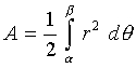
Let  r = f(q) define a polar curve, where f is continuous and f(q) > 0 on the closed interval a < q < b  for 0 < b - a < 2p.  Then the region bounded by the curve r = f(q) and the rays q = a and q = b has area:

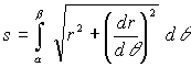
The arc length of a polar curve r = f(q) for a < q < b is given by the integral:

Find the arc length and the area of the cardioid defined in part (A).

>  restart;
>  with(plots):
>  r := 1 + cos(theta);
>  areaCardioid := (1/2)* int (r^2, theta = 0..2*Pi);
>  evalf(%);
>  arcLengthCardioid := int ( sqrt(r^2 +  diff(r, theta)^2) ,  theta);

Exercises:

1.   Find the area of Pascal's limacon.
2.   Find the arc length of Archimedes' spiral from theta = 0 to 13 radians.

(C)   Point on a graph.

There are several ways to specify one or more points on a graph.  For example, let us consider the graph of the parabola y = x² and the points P = (2,4) and Q = (3,9).

> parabolaGraph := plot(x^2, x = 0..3.5):
> L := [[2,4], [3,9]];   #  this is our list of points
> pointsPandQ := plot(L, style = point, symbol = circle, color = BLACK);
> display ({parabolaGraph, pointsPandQ});

Of course, we can improve upon the appearance of the graph by adding text near the two points of interest:

>  pointText := textplot( [ [2.5, 4, `P=(2,4)`], [3.5, 9, `Q=(3,9)`] ]):
> display ({parabolaGraph, pointsPandQ, pointText});

(As an alternative approach one could simply place Xs at the location of the points by using the textplot command.)

Next, let us find the points of intersection of the circle (in polar form) r = sin q and the spiral r = q.

>  restart:
>  with(plots):
>  rCircle := 5*sin(theta);
>  circlePlot := polarplot( rCircle, theta = 0..2*Pi, color = GREEN):

>  rSpiral := theta;
>  spiralPlot := polarplot( rSpiral, theta = 0..2*Pi, color = RED):

>   display ({circlePlot, spiralPlot});

Clearly one point of intersection is the origin.  The other may be found using the fsolve command:

>  thetaIntersection := fsolve (rCircle = rSpiral, theta = 0.1..2*Pi);
>  rIntersection := subs( theta = thetaIntersection, rCircle);

Next, the point of intersection that was found in polar coordinates must now be converted to Cartesian coordinates using the relationship x = r cos q and y = r sin q.

>   xInter := rIntersection * cos(thetaIntersection);
>   yInter := rIntersection * sin(thetaIntersection);
>   L := [[xInter, yInter], [0,0]];    #  These are our two points of intersection expressed in Cartesian coordinates.
>   pointsOfIntersection := plot( L, style = point, symbol = circle, color = BLACK):
>   display ({circlePlot, spiralPlot, pointsOfIntersection});

Exercise:   Add an appropriate title and appropriate text to the graph above that labels the coordinates of the two points of intersection.

(D)  Piecewise linear continuous functions.

In Maple it is quite easy to graph a function that is formed by connecting, in a linear manner, a finite set of points.  For example:

>  L := [ [0,0], [1,1], [2,4], [4,0], [7,-3] ];
>   plot (L);

Exercise:  Experiment with this feature by creating a few examples of your own.

(E)   Graphing solids of revolution.

In Maple 8, the Calculus1 package of the Student library makes it very easy to graph a solid of revolution that has as its axis of revolution either the x-axis or the y-axis.

For example:

>  with(Student[Calculus1]):
>  VolumeOfRevolution( sin(x)^3 , x = 0..Pi, output = plot, axis = vertical);
>  VolumeOfRevolution( sin(x)^3 , x = 0..Pi, output = plot, axis = horizontal);
>  VolumeOfRevolution(1+cos(x), x = 0..4*Pi, output=plot, axis = horizontal);
>  VolumeOfRevolution(1+cos(x), x = 0..4*Pi, output=plot, axis = vertical);
>  VolumeOfRevolution(ln(x), x = 1..3, output=plot, axis = horizontal);
>  VolumeOfRevolution(ln(x), x = 1..3, output=plot, axis = vertical);
>  VolumeOfRevolution(4*x, x,  x = 0..1, output=plot, axis = vertical);  #  Here we view the solid obtained by rotating the region bounded by y = 4x and y = x from x=0 to x=1.

Exercise: Consider the region bounded by the curves y = x²  and y = x³.  Rotate this region about each of the coordinate axes.