Class Notes – Wednesday 25 January 2006

Continuation of ANOCOV

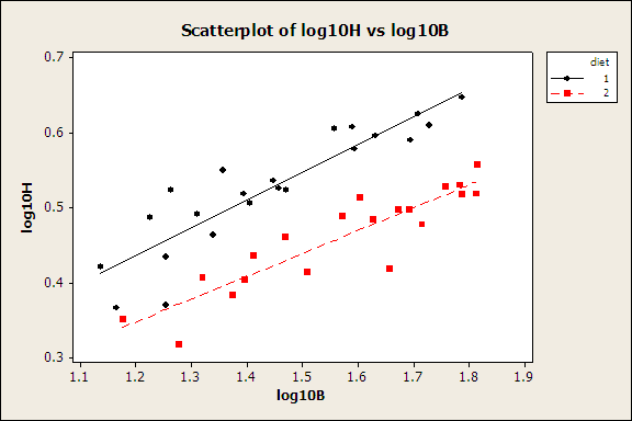
· This graph illustrates the parallelism detected on p.12;

• We really have no business performing an ANOCOV analysis if we cannot accept parallelism; parallelism means that the covariate affects the response variable in a similar manner for the two drugs or groups, etc.;
• Homework 1 ex. 1 demonstrates the importance of first removing covariate(s) (i.e., doing ANOCOV) before comparing means of Y, as opposed to just doing a simple 2-sample t-test (and ignoring the covariate);
• In the presence of an interaction term, main-effects terms cannot be interpreted and are meaningless.

New Section 2.6 Material

· Sometimes the Wald procedure on a transformed scale yields reliable CI’s, and sometimes we have to go to the trouble to find the more reliable likelihood-based CI’s;

· Examples include the CC (correlation coefficient) even when normality is assumed, and also p, OR, and RR (latter 3 are in the Appendix);

· Fisher showed a good transformed scale for the CC (r) is the inverse hyperbolic tangent, k = ½log{(1+r)/(1-r)}, from which we get the CI given in (6.7);

· For the CC, the likelihood-based CI is given in (6.9);

· For the original Efron GPA data graphed on p.14 (n=15), these two intervals are close (top of p.15) for both 95% and 99%, and graphs in mid-p.15 are close;

· This breaks down for small samples: note the big difference between the two 95% CI’s for data graphed on p.16 (n=6) – graphs differ a lot on p.16;

· When do Wald methods break down? This is a function of the model/data curvature;

· Bottom line: likelihood methods are usually preferred, but computationally more work.

Examples in the Appendix

Again, there exist modified Wald-type intervals which – for large sample sizes – approximate the likelihood intervals.