Advanced
Biostatistics Homework 1 Due: 1st February 2006
Directions: Answer the parts of the following four exercises, showing all relevant work. Attach computer output only as necessary. Conclusions and justifications are to be given in clear detailed English. Please type up your solutions or write very neatly.
1. Norman & Streiner report
(p.146) the medical data set reproduced below.
Analyze these data by performing each of the following analyses. In each
case, list all necessary assumptions, and clearly summarize your conclusions.
Subject |
1 |
2 |
3 |
4 |
5 |
6 |
7 |
8 |
9 |
10 |
11 |
12 |
13 |
14 |
15 |
16 |
|
Y |
46 |
36 |
40 |
44 |
36 |
30 |
42 |
35 |
42 |
50 |
45 |
53 |
48 |
38 |
43 |
58 |
|
Treatment |
A |
A |
B |
A |
A |
B |
A |
B |
B |
A |
A |
B |
B |
B |
B |
A |
|
X |
12 |
14 |
27 |
35 |
26 |
21 |
48 |
51 |
62 |
64 |
60 |
77 |
91 |
84 |
55 |
74 |
(a) [All students] Perform two independent sample t-tests
(one assuming equal variances and one assuming unequal variances) comparing the
Y averages for the two treatment groups.
(b) [All students] Regress Y on X, obtain parameter estimates,
and test whether X is a good predictor of Y.
(c) [G students only] Perform the ANOCOV (Analysis of covariance)
analysis to determine if the Y averages differ for the two treatment group
after removing the effect of X.
2. [All Students]
Extracorporeal membrane oxygenation (ECMO) is a potentially life-saving
procedure that is used to treat newborn babies who suffer from severe
respiratory failure. An experiment was
conducted in which 20 babies were treated with ECMO and 30 babies were treated
with conventional medical therapy (CMT).
At the end of the study, 11 of the CMT babies died (19 survived), and
only 2 of the ECMO babies died (18 survived).
(a) Test whether these data
suggest that the therapies significantly differ.
(b) Find and interpret the Odds
Ratio (OR) of survival comparing the ECMO therapy with the CMT, and provide a
95% confidence interval for the true OR.
(c) Let’s alter the above data
by supposing that of the 20 ECMO babies, none died (all 20 survived). Explain why the usual (chi-square) test
statistic is inappropriate here, and analyze the (new) data using the correct
analysis.
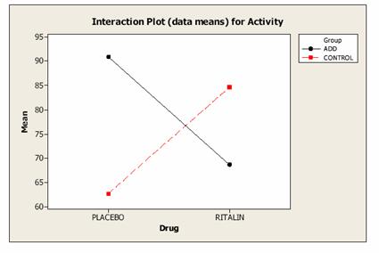
3. [G students only] Two groups of children, one with attention
deficit disorder (ADD) and a control group of children without ADD, were
randomly given either a placebo or the drug Ritalin. A measure of activity was made on all the
children with the results shown in the table below (higher numbers indicate
more activity). Analyze these data
(listing all necessary assumptions), including all relevant observations and
implications.
|
Treatment |
Group |
Drug |
Activity |
|
1 |
ADD |
PLACEBO |
90 |
|
1 |
ADD |
PLACEBO |
88 |
|
1 |
ADD |
PLACEBO |
95 |
|
2 |
CONTROL |
PLACEBO |
60 |
|
2 |
CONTROL |
PLACEBO |
62 |
|
2 |
CONTROL |
PLACEBO |
66 |
|
3 |
ADD |
RITALIN |
72 |
|
3 |
ADD |
RITALIN |
70 |
|
3 |
ADD |
RITALIN |
64 |
|
4 |
CONTROL |
RITALIN |
86 |
|
4 |
CONTROL |
RITALIN |
86 |
|
4 |
CONTROL |
RITALIN |
82 |
4. (
|
Sub |
1 |
2 |
3 |
4 |
5 |
6 |
7 |
8 |
9 |
10 |
11 |
12 |
13 |
14 |
15 |
16 |
17 |
18 |
|
PreW |
165 |
202 |
256 |
155 |
135 |
175 |
180 |
174 |
136 |
168 |
207 |
155 |
220 |
163 |
159 |
253 |
138 |
287 |
|
PostW |
160 |
200 |
259 |
156 |
134 |
162 |
187 |
172 |
138 |
162 |
197 |
155 |
205 |
153 |
150 |
255 |
128 |
280 |
|
Sub |
19 |
20 |
21 |
22 |
23 |
24 |
25 |
26 |
27 |
28 |
29 |
30 |
31 |
32 |
33 |
34 |
35 |
|
|
PreW |
177 |
181 |
148 |
167 |
190 |
165 |
155 |
153 |
205 |
186 |
178 |
129 |
125 |
165 |
156 |
170 |
145 |
|
|
PostW |
171 |
170 |
154 |
170 |
180 |
154 |
150 |
145 |
206 |
184 |
166 |
132 |
127 |
169 |
158 |
161 |
152 |
|
(a) [All Students] Does the new treatment look at all
promising? Be specific and list all
necessary assumptions and/or reasons why some usual one(s) are not needed here.
(b) [All Students]
Does a subjects’ “Pre” weight appear to be a good linear predictor of
his/her “Post” weight? Again, be
specific and list all necessary assumptions and/or reasons why some usual
one(s) are not needed here.
(c) [G Students only] Reconcile the analyses in parts (a) and
(b). That is, discuss any connection(s)
(if any) between the two analyses.
Homework 1 Attachment –
Minitab Output
Exercise
1(a)
|
Two-Sample T-Test and CI: y, trt Two-sample T for y trt N Mean
StDev SE Mean a 8 44.63 7.23 2.6 b 8 41.13 7.22 2.6 Difference = mu (a) - mu (b) Estimate for difference: 3.50 95% CI for difference:
(-4.25, 11.25) T-Test of difference = 0
(vs not =): T-Value = 0.97 P-Value =
0.349 DF = 14 Both use Pooled StDev =
7.22 Two-Sample T-Test and CI: y, trt Two-sample T for y trt N Mean
StDev SE Mean a 8 44.63 7.23 2.6 b 8 41.13 7.22 2.6 Difference = mu (a) - mu
(b) Estimate for difference: 3.50 95% CI for difference:
(-4.30, 11.30) T-Test of difference = 0 (vs not =): T-Value = 0.97 P-Value = 0.350 DF = 13 |
Exercise
1(b)
Regression
Analysis: y versus x
The regression equation is y = 35.0 + 0.158 x Predictor Coef SE Coef T P Constant 34.978 3.553 9.84
0.000 x 0.15774
0.06381 2.47 0.027 S = 6.227 R-Sq = 30.4% R-Sq(adj) = 25.4% Analysis of Variance Source DF SS MS F P Regression 1 236.94 236.94 6.11
0.027 Residual Error 14
542.81 38.77 Total |
Exercise
1(c)
|
Regression Analysis: y versus x,
dum, dumx The regression equation is y = 35.1 + 0.228 x - 5.09
dum - 0.039 dumx Predictor Coef SE Coef T P Constant 35.127 4.192 8.38
0.000 x 0.22819 0.08908 2.56
0.025 dum -5.093 6.673 -0.76
0.460 dumx -0.0386 0.1212 -0.32
0.756 S = 5.532 R-Sq = 52.9% R-Sq(adj) = 41.1% Analysis of Variance Source DF SS MS F P Regression 3 412.55 137.52 4.49
0.025 Residual Error 12
367.20 30.60 Total 15 779.75 |
|
Regression Analysis: y versus x,
dum The regression equation is y = 36.0 + 0.207 x - 7.00
dum Predictor Coef SE Coef T P Constant 35.994 3.074 11.71
0.000 x 0.20735 0.05829 3.56
0.004 dum -6.999 2.844
-2.46 0.029 S = 5.337 R-Sq = 52.5% R-Sq(adj) = 45.2% Analysis of Variance Source DF SS MS F P Regression 2 409.45 204.72 7.19
0.008 Residual Error 13
370.30 28.48 Total 15 779.75 |
Exercise
2(a)
|
Chi-Square Test: CMT, ECMO Expected counts are printed
below observed counts ECMO CMT
Total 1
18 19 37 14.80 22.20 2
2 11 13 5.20 7.80 Total 20 30 50 Chi-Sq = 0.692 +
0.461 + 1.969 + 1.313 = 4.435 DF = 1, P-Value = 0.035 |
Exercise
3
|
Two-way ANOVA: activity versus
group, drug Analysis of Variance for
activity Source DF
SS MS F P group 1 114.1
114.1 10.14 0.013 drug 1 0.1 0.1
0.01 0.934 Interaction 1
1474.1 1474.1 131.03
0.000 Error 8 90.0 11.3 Total 11 1678.3 |
Exercise
4(a)
|
Paired T-Test and CI: wtpre,
wtpost Paired T for wtpre - wtpost N Mean
StDev SE Mean wtpre 35 174.94
35.94 6.07 wtpost 35 171.49
35.45 5.99 Difference 35
3.46 6.34 1.07 95% lower bound for mean
difference: 1.65 T-Test of mean difference = 0 (vs > 0): T-Value = 3.23 P-Value = 0.001 |
Exercise
4(b)
|
Regression Analysis: wtpost versus
wtpre The regression equation is wtpost = 1.61 + 0.971 wtpre Predictor Coef SE Coef T P Constant 1.615 5.407 0.30
0.767 wtpre 0.97101 0.03030 32.05
0.000 S = 6.348 R-Sq = 96.9% R-Sq(adj) = 96.8% Analysis of Variance Source DF SS MS F P Regression 1 41397 41397
1027.31 0.000 Residual Error 33
1330 40 Total 34 42727 Unusual Observations Obs wtpre wtpost Fit SE Fit Residual St Resid 3
256 259.00 250.19 2.68 8.81 1.53 X 18
287 280.00 280.29 3.56 -0.29 -0.06 X X denotes an observation whose X value gives it large influence. |