Advanced
Biostatistics Homework 1 Solutions Due: 1st February 2006
Directions: Answer the parts of the following four exercises, showing all relevant work. Attach computer output
only as necessary. Conclusions and justifications are to be given in clear detailed English. Please type up your solutions.
1. Norman & Streiner report
(p.146) the medical data set reproduced below.
Analyze these data by performing each
of the following analyses. In
each case, list all necessary assumptions, and clearly summarize your
conclusions.
Subject |
1 |
2 |
3 |
4 |
5 |
6 |
7 |
8 |
9 |
10 |
11 |
12 |
13 |
14 |
15 |
16 |
|
Y |
46 |
36 |
40 |
44 |
36 |
30 |
42 |
35 |
42 |
50 |
45 |
53 |
48 |
38 |
43 |
58 |
|
Treatment |
A |
A |
B |
A |
A |
B |
A |
B |
B |
A |
A |
B |
B |
B |
B |
A |
|
X |
12 |
14 |
27 |
35 |
26 |
21 |
48 |
51 |
62 |
64 |
60 |
77 |
91 |
84 |
55 |
74 |
(a) [All students] Perform two independent sample t-tests
(one assuming equal variances and one assuming unequal
variances) comparing the Y averages
for the two treatment groups.
Assuming unequal
variances
Two-Sample T-Test and CI: y, trt Two-sample T for y trt N Mean
StDev
SE Mean a 8 44.63 7.23 2.6 b 8 41.13
7.22 2.6 Difference = mu (a) - mu (b) Estimate for
difference: 3.50 95% CI for difference:
(-4.30, 11.30) T-Test of difference = 0 (vs not =): T-Value = 0.97
P-Value = 0.350
DF = 13 |
Assuming equal variances
Two-Sample T-Test and CI: y, trt Two-sample T for y trt N Mean
StDev
SE Mean a 8 44.63 7.23 2.6 b 8 41.13 7.22 2.6 Difference = mu (a) - mu (b) Estimate for
difference: 3.50 95% CI for difference:
(-4.25, 11.25) T-Test of difference = 0 (vs not =): T-Value = 0.97
P-Value = 0.349
DF = 14 Both use Pooled StDev = 7.22 |
We note from each
of the above outputs that we would retain the null hypothesis of equality of
the two Y means
(for
the two drugs) with respective p-values of 35.0% and 34.9% respectively. This conclusion is based on
assumptions of normality of the respective parent
populations, random samples (independence, representative,
absence of bias), and equal variances for the first
test.
(b) [All students] Regress Y on X, obtain parameter estimates,
and test whether X is a good predictor of Y.
Regression
Analysis: y versus x
The regression equation is y = 35.0 + 0.158 x Predictor Coef SE Coef T P Constant 34.978
3.553 9.84
0.000 x 0.15774 0.06381 2.47
0.027 S = 6.227 R-Sq = 30.4% R-Sq(adj) =
25.4% Analysis of Variance Source DF SS MS F P Regression 1 236.94
236.94 6.11
0.027 Residual Error 14
542.81 38.77 Total |
Noting that the p-value
associated with the test of H0: b1
= 0 (in the SLR model Ey = b0 + b1x)
is 2.7%
(less
than a = 5%), meaning that we reject this null
hypothesis, and conclude that X is indeed a good
linear predictor of Y. This test is based on the assumption of
normality, constant variance, a random
sample, and the assumption of a linear
relationship between Y and X.
(c) [G students only] Perform the ANOCOV (Analysis of covariance)
analysis to determine if the Y averages
differ for the two treatment group
after removing the effect of X.
First
ensure that lines are parallel (first MLR), then test whether drug averages
differ after adjusting for X.
|
Regression Analysis: y versus x, dum, dumx The regression equation is y = 35.1 + 0.228 x - 5.09 dum - 0.039 dumx Predictor Coef SE Coef T P Constant 35.127 4.192 8.38
0.000 x 0.22819 0.08908 2.56
0.025 dum -5.093 6.673 -0.76
0.460 dumx -0.0386 0.1212 -0.32
0.756 S = 5.532 R-Sq = 52.9% R-Sq(adj) =
41.1% Analysis of Variance Source DF SS MS F P Regression 3 412.55 137.52 4.49
0.025 Residual Error 12
367.20 30.60 Total 15 779.75 |
|
Regression Analysis: y versus x, dum The regression equation is y = 36.0 + 0.207 x - 7.00 dum Predictor Coef SE Coef T P Constant 35.994 3.074 11.71
0.000 x 0.20735 0.05829 3.56
0.004 dum -6.999 2.844 -2.46
0.029 S = 5.337 R-Sq = 52.5% R-Sq(adj) =
45.2% Analysis of Variance Source DF SS MS F P Regression 2 409.45 204.72 7.19
0.008 Residual Error 13
370.30 28.48 Total 15 779.75 |
Note first
that the interaction term (called “dumx”) in the
first MLR model can be dropped, prompting
us to accept the necessary assumption of
parallelism, and to proceed to the ANOCOV (second regression).
For
the latter regression (which controls for the covariate X), these data give
evidence of a difference
between the averages for the two drugs. The assumptions here are as above in (b) plus
the parallelism assumption.
2. [All Students]
Extracorporeal membrane oxygenation (ECMO) is a potentially life-saving
procedure that is used
to treat newborn babies who
suffer from severe respiratory failure.
An experiment was conducted in which 20 babies
were treated with ECMO and 30
babies were treated with conventional medical therapy (CMT). At the end of the
study, 11 of the CMT babies died
(19 survived), and only 2 of the ECMO babies died (18 survived).
(a) Test whether these data
suggest that the therapies significantly differ.
|
Chi-Square Test: CMT, ECMO Expected counts are printed
below observed counts ECMO CMT
Total 1
18 19 37 14.80 22.20 2
2
11 13 5.20 7.80 Total 20 30 50 Chi-Sq = 0.692 +
0.461 + 1.969 + 1.313 = 4.435 DF = 1, P-Value = 0.035 |
The
null hypothesis that is tested here is that the therapies have the same
survival rate, and this hypothesis is
rejected (p = 3.5%) at the 5% level, thereby
suggesting that the therapies differ in their survival rates (ECMO
has a significantly higher survival rate).
(b) Find and interpret the Odds
Ratio (OR) of survival comparing the ECMO therapy with the CMT, and provide
a 95% confidence interval for
the true OR.
The estimated OR is (18*11)/(2*19) = 5.2105, the estimated (natural) log-OR is
1.650680871, and the estimated
SE is SQRT{1/18
+ 1/19 + 1/2 + 1/11} = 0.83612. The 95%
CI for the log-OR is 1.6507 +/- 1.96*0.83612
= 1.6507 +/- 1.6388 = (0.011886 , 3.28948).
Exponentiating these limits gives us an approximate 95% CI for the
OR of (1.012,26.829). Since this
CI significantly exceeds unity (1), we conclude that the odds of survival for
the
ECMO significantly exceeds
the odds of survival for the CMT therapy.
Specifically, these data suggest that the
Odds of survival for the
ECMO group is at least 1.012 times the odds of survival for the CMT group (and
at most
26.829 times).
(c) Let’s alter the above data
by supposing that of the 20 ECMO babies, none died (all 20 survived). Explain why the
usual (chi-square) test statistic
is inappropriate here, and analyze the (new) data using the correct analysis.
Note that in the
original 2x2 table, all the expected cell counts were at least 5, and thus we
were justified in using
the chi-square test. In contrast, for the new 2x2 table, one of
the expected cell counts is less than 5 (4.4 for the 0 cell),
and so we must use Fisher’s Exact Test
(FET). In the sense of this test, there
is no table more extreme than the
realized one, and note that the p-value associated
is therefore 39C20*11C0/50C20
= 0.001462432 (from S-Plus).
Again, we reject
the null hypothesis and conclude as in part (a).
3. [G students only] Two groups of children, one with attention
deficit disorder (ADD) and a control group of children
without ADD, were randomly given
either a placebo or the drug Ritalin. A
measure of activity was made on all the
children with the results shown in
the table below (higher numbers indicate more activity). Analyze these data (listing
all necessary assumptions),
including all relevant observations and implications.
|
Treatment |
Group |
Drug |
Activity |
|
1 |
ADD |
PLACEBO |
90 |
|
1 |
ADD |
PLACEBO |
88 |
|
1 |
ADD |
PLACEBO |
95 |
|
2 |
CONTROL |
PLACEBO |
60 |
|
2 |
CONTROL |
PLACEBO |
62 |
|
2 |
CONTROL |
PLACEBO |
66 |
|
3 |
ADD |
RITALIN |
72 |
|
3 |
ADD |
RITALIN |
70 |
|
3 |
ADD |
RITALIN |
64 |
|
4 |
CONTROL |
RITALIN |
86 |
|
4 |
CONTROL |
RITALIN |
86 |
|
4 |
CONTROL |
RITALIN |
82 |
|
Two-way ANOVA: activity versus
group, drug Analysis of Variance for
activity Source DF SS MS F P group 1 114.1
114.1
10.14 0.013 drug 1 0.1
0.1
0.01 0.934 Interaction 1
1474.1 1474.1 131.03
0.000 Error 8 90.0 11.3 Total 11
1678.3 |
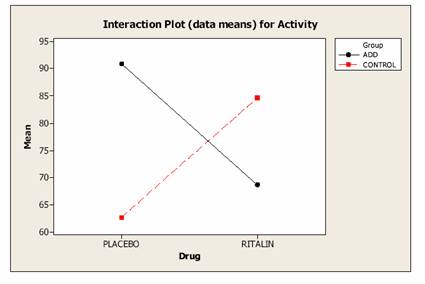
These data provide
good evidence of an interaction between Drug and patient Group, meaning that the
effect
of Ritalin depends upon whether the patient is
in the ADD group or the Control group.
It turns out that Ritalin
has a significant dampening effect on activity
for the ADD group and a significant stimulating effect on the
Control group. These tests are predicated upon the normality
assumption with equal variances, and absence
of bias, independence, representative samples
(random sampling).
4. (
A preliminary study of 35 obese patients provided
the following data on patients’ body weights (in pounds) before
(“PreW”,
in pounds) and after (“PostW”, in pounds) 10 weeks of
treatment with the new compound.
|
Sub |
1 |
2 |
3 |
4 |
5 |
6 |
7 |
8 |
9 |
10 |
11 |
12 |
13 |
14 |
15 |
16 |
17 |
18 |
|
PreW |
165 |
202 |
256 |
155 |
135 |
175 |
180 |
174 |
136 |
168 |
207 |
155 |
220 |
163 |
159 |
253 |
138 |
287 |
|
PostW |
160 |
200 |
259 |
156 |
134 |
162 |
187 |
172 |
138 |
162 |
197 |
155 |
205 |
153 |
150 |
255 |
128 |
280 |
|
Sub |
19 |
20 |
21 |
22 |
23 |
24 |
25 |
26 |
27 |
28 |
29 |
30 |
31 |
32 |
33 |
34 |
35 |
|
|
PreW |
177 |
181 |
148 |
167 |
190 |
165 |
155 |
153 |
205 |
186 |
178 |
129 |
125 |
165 |
156 |
170 |
145 |
|
|
PostW |
171 |
170 |
154 |
170 |
180 |
154 |
150 |
145 |
206 |
184 |
166 |
132 |
127 |
169 |
158 |
161 |
152 |
|
(a) [All Students] Does the new treatment look at all
promising? Be specific and list all
necessary assumptions and/or
reasons why some usual one(s) are
not needed here.
|
Paired T-Test and CI: wtpre, wtpost Paired T for wtpre - wtpost N Mean
StDev
SE Mean wtpre 35 174.94
35.94 6.07 wtpost 35 171.49
35.45 5.99 Difference 35
3.46 6.34 1.07 95% lower bound for mean
difference: 1.65 T-Test of mean difference =
0 (vs > 0): T-Value = 3.23 P-Value = 0.001 |
These data provide evidence
of a significant drop in body weight after use of the new compound. Since the sample
size is large, we do not need to assume
normality of the distribution of differences in weight, but we do need to
assume
that the sample was random (independence, that
the sample is representative, no bias).
(b) [All Students] Does a subjects’ “Pre” weight appear to be a
good linear predictor of his/her “Post” weight?
Again,
be specific and list all
necessary assumptions and/or reasons why some usual one(s) are not needed here.
|
Regression Analysis: wtpost versus wtpre The regression equation is wtpost = 1.61 + 0.971 wtpre Predictor Coef SE Coef T P Constant 1.615 5.407 0.30
0.767 wtpre 0.97101 0.03030 32.05
0.000 S = 6.348 R-Sq = 96.9% R-Sq(adj) =
96.8% Analysis of Variance Source DF SS MS F P Regression 1 41397 41397 1027.31
0.000 Residual Error 33
1330 40 Total 34 42727 Unusual Observations Obs wtpre wtpost Fit SE Fit Residual St Resid 3
256 259.00 250.19 2.68 8.81 1.53 X 18
287 280.00 280.29 3.56 -0.29 -0.06 X X denotes an observation
whose X value gives it large influence. |
Yes, the “Pre” weight does appear to
be a good linear predictor of the “Post” weight (t = 32.05, p = 0.000)
subject to the assumptions of normality, equal
variances, and a random sample (no bias, etc.).
(c) [G Students only] Reconcile the analyses in parts (a) and
(b). That is, discuss any connection(s)
(if any)
between the two analyses.
The paired t-test is equivalent to SL regression with the insistence that
b1
= 1 and which then tests whether
the intercept is zero. SLR, on the other hand, allows the slope to
vary from unity. We hasten to add that the
assumptions for
the SLR are more stringent than for the paired t-test.